
Static Pressure
To supplement our discussion of the Reynolds number and as a prelude to the polar diagram, today we will examine the forces acting on the airfoil that result from the air mass and airspeed. An important phenomenon affecting the airfoil is dynamic pressure.
During level flight, the lift generated by the wing must equal the model’s weight. The airflow must perform a lifting force every second to support the model; otherwise, it would transition into a glide, during which the kinetic energy of the air at the wing profile is converted into pressure energy. The kinetic energy contained in one cubic meter of moving air—work capacity or kinetic energy—is equal to the dynamic pressure $q$, which plays the primary role as the most important aerodynamic unit of measurement in all calculations of aerodynamic forces and velocity.
From mechanics, we know the fundamental law:
"Kinetic energy is equal to the product of mass ($M$) and the square of velocity ($v^2$), divided by 2," written as a formula:
$$\text{Kinetic energy} = \frac{M \cdot v^2}{2} \quad (\text{kilogram-ster})$$
However, since the mass of 1 cubic meter of air is equal to the air density $\epsilon$, substituting this for $M$ yields:
$$\text{Kinetic energy} = \frac{\epsilon \cdot v^2}{2} = \text{Dynamic pressure } q \quad (\text{kg/m}^2)$$
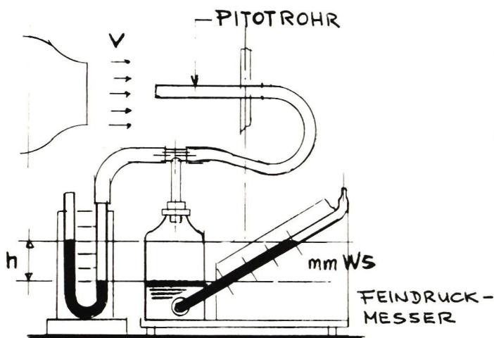
The dynamic pressure accumulated in the Pitot tube is read in millimeters of water column on the U-tube manometer. When using alcohol as the filling fluid—which is the recommended method—$h$ is multiplied by the density of alcohol (0.8). For the low pressures being measured here, the reading on the high-precision pressure gauge is more accurate. The more the inclined tube is tilted, the larger the pressure reading appears on the scale; for example, here it is doubled.
Procedure:
If we blow air in a free jet from an air generator into an open tube connected to a pressure gauge via a rubber hose, the air is compressed within the tube, thereby converting the kinetic energy contained in the air mass into pressure energy. The height of the vertical water column $h$ resulting from the increased pressure is a measure of the dynamic pressure (more precisely: $h$ is a measure of the total pressure $P = q + p$. However, since in a free jet the static pressure $p = 0$, or is equal to the pressure in free space, the total pressure $P$ can be set equal to the dynamic pressure $q$ here.), and specifically, $h = 1 \text{ mm water column} = 1 \text{ kg/m}^2$ of dynamic pressure, because a volume of water with a base area of $1 \text{ m}^2$ and a height of $1 \text{ mm}$ weighs $1 \text{ kg}$ .
The dynamic pressure therefore increases with air density and the square of the velocity. For standard atmospheric conditions ($15^\circ \text{C}$ and $760 \text{mm QS}$) at an altitude of zero meters, $\epsilon = 1/8$. For model flight near the ground, the simplified formula is therefore sufficient:
$$q = \frac{1 \cdot v^2}{8 \cdot 2} = \frac{v^2}{16} \quad \text{kg/m}^2$$
In a model aircraft flight measurement, a model glides $48 \text{ m}$ in still air in $8 \text{ seconds}$. Calculate the speed and the dynamic pressure.
$$\begin{aligned} \text{Velocity} \quad v &= 48 : 8 = 6 \text{ m/sec} \\ \text{Dynamic pressure} \quad q &= v^2 / 16 = 6 \cdot 6 / 16 = 2.25 \text{ kg/m}^2 \end{aligned}$$
$$\text{Velocity} \quad v = 4 \sqrt{q} \quad (\text{m/s})$$
If the dynamic pressure is given, the velocity is calculated using the following formula:
$$\text{Velocity: } v = \sqrt{\frac{2}{\epsilon}} q$$
$$\text{For a height of zero meters: } v = \sqrt{\frac{2}{\frac{1}{8}}} q = 4 \sqrt{q}$$
Calculate the velocity for the two notable dynamic pressures $q = 1 \text{ kg/m}^2$ and $16 \text{ kg/m}^2$.
For $q = 1$, $v = 4\sqrt{1} = 4 \text{ m/sec}$
$q = 16$, $v = 4\sqrt{16} = 16 \text{ m/sec}$
For $v = 0$ to $16 \text{ m/s}$, the corresponding dynamic pressure can be read from Figure B. Any quadratic law results in a parabola when plotted graphically.
We will need the practical application of this theoretical discussion later when calculating the model velocity. Heinrich Disler
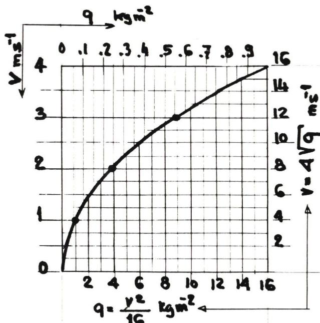
| q (kg/m²) | v (m/s) |
|---|---|
| 0 | 0 |
| 1 | 4 |
| 4 | 8 |
| 9 | 12 |
| 16 | 16 |


News from HEBU

TEAM MANAGER "THIS" BOSSHARD
 Rodito Nussbaumer
YOU KNOW WHAT I MEAN? 125 YEARS OF THE SWISS AERO CLUB
 Emil Giezendanner

PRIDE AND GOOD IDEAS
 Markus Nussbaumer
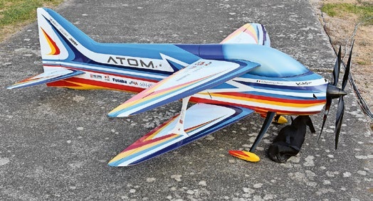
ATOM, THE NEW DOUBLE-DECKER FROM CPLR
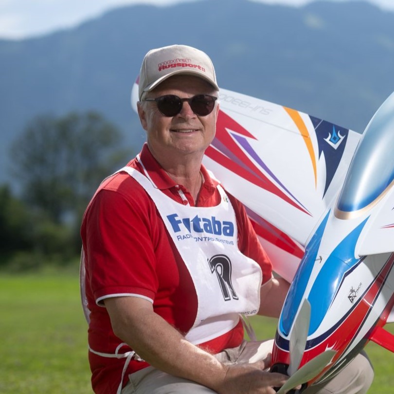 Matthias Bosshard

SUMMER FUN 2026 AT MG USTER
Martin Wunderli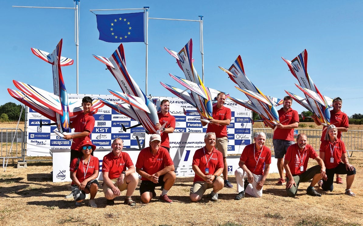
F3A EUROPEAN CHAMPIONSHIPS IN ST-MACAIRE, FRANCE
Matthias Bosshard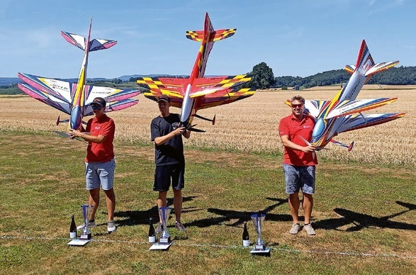
52. 2026 ALPS CUP
Emil Giezendanner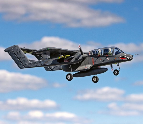
HORIZON HOBBY/LEMACO NEWS: MICRO OV-10 BRONCO 645 MM BY E-FLITE
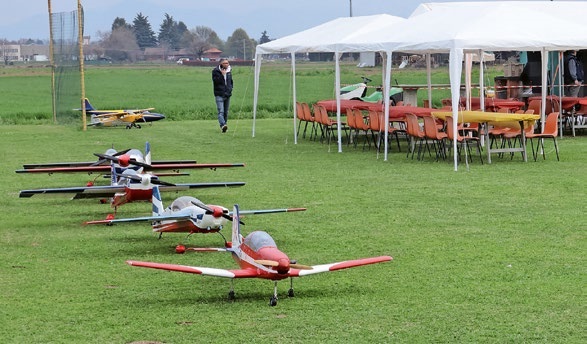
TWIN TOWN PARTNERSHIP
Wolfgang Voeller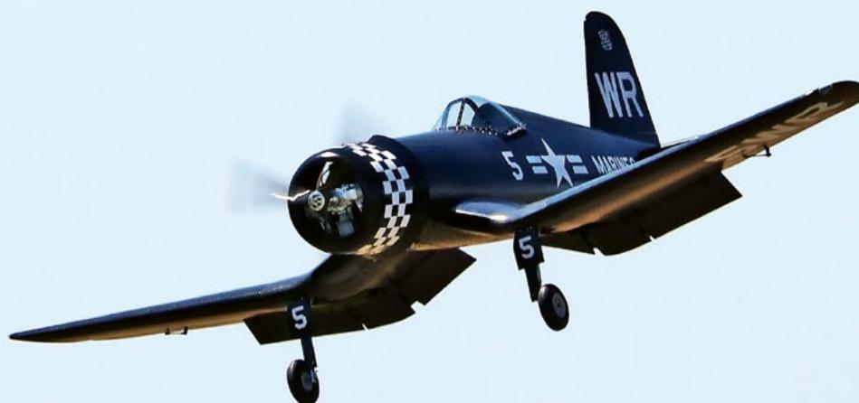
CORSAIR F4U – A WARBIRD WITH A MEMORABLE LOOK
Jürgen Rosenberger, Jürgen Prinz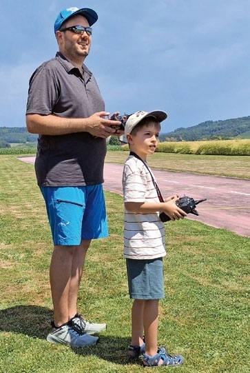
TRY-OUT DAY AT MFV WETTINGEN
Urs Keller
EURO CONTEST GLIDER ACRO TOUR AUSTRIA 2026
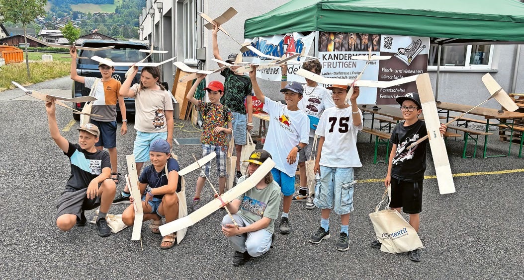
BY YOUTH, FOR YOUTH
Lorena Betschen
INSIGHTS INTO THE HISTORY OF SEAPLANES
SMALL, MODEL-LIKE SAILBOATS
Res Dauwalder
What's New at Leomotion.com
COUPE DES ALPES – OBSERVE AND LEARN
Rodito Nussbaumer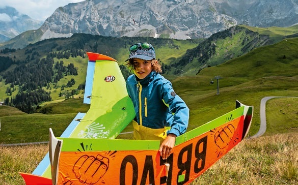
34th HAHNENMOOS ALPINE MODEL AIRPLANE CAMP
Res Dauwalder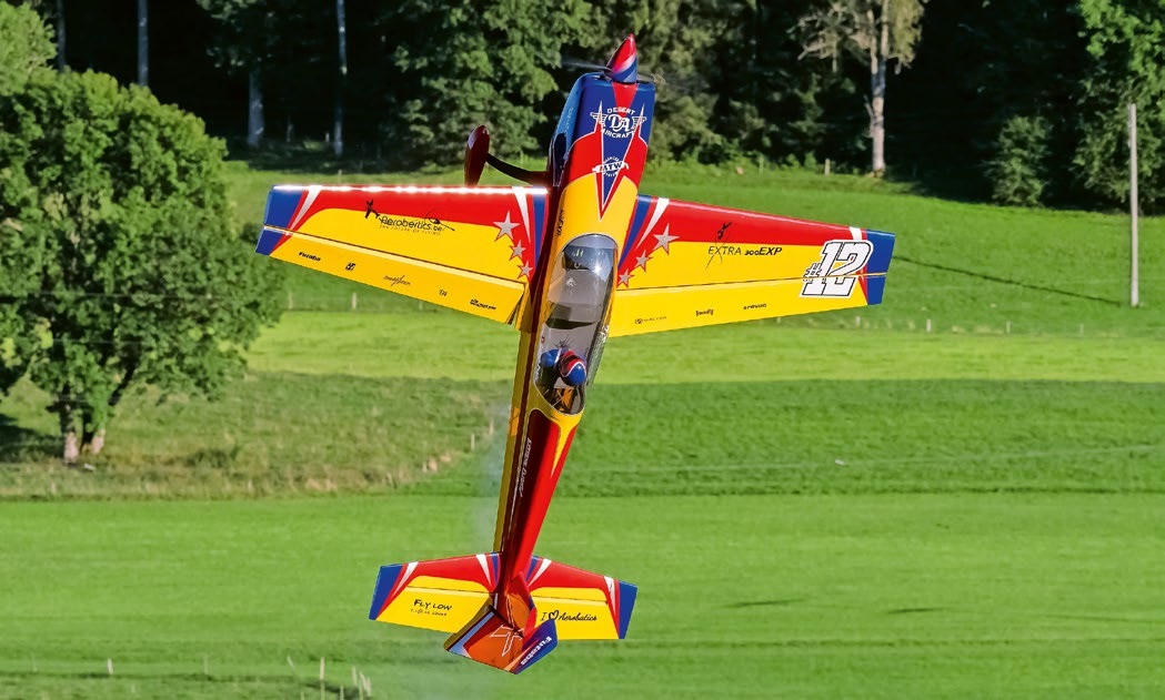
WELCOME, NEW MEMBER!
Andrea Bolliger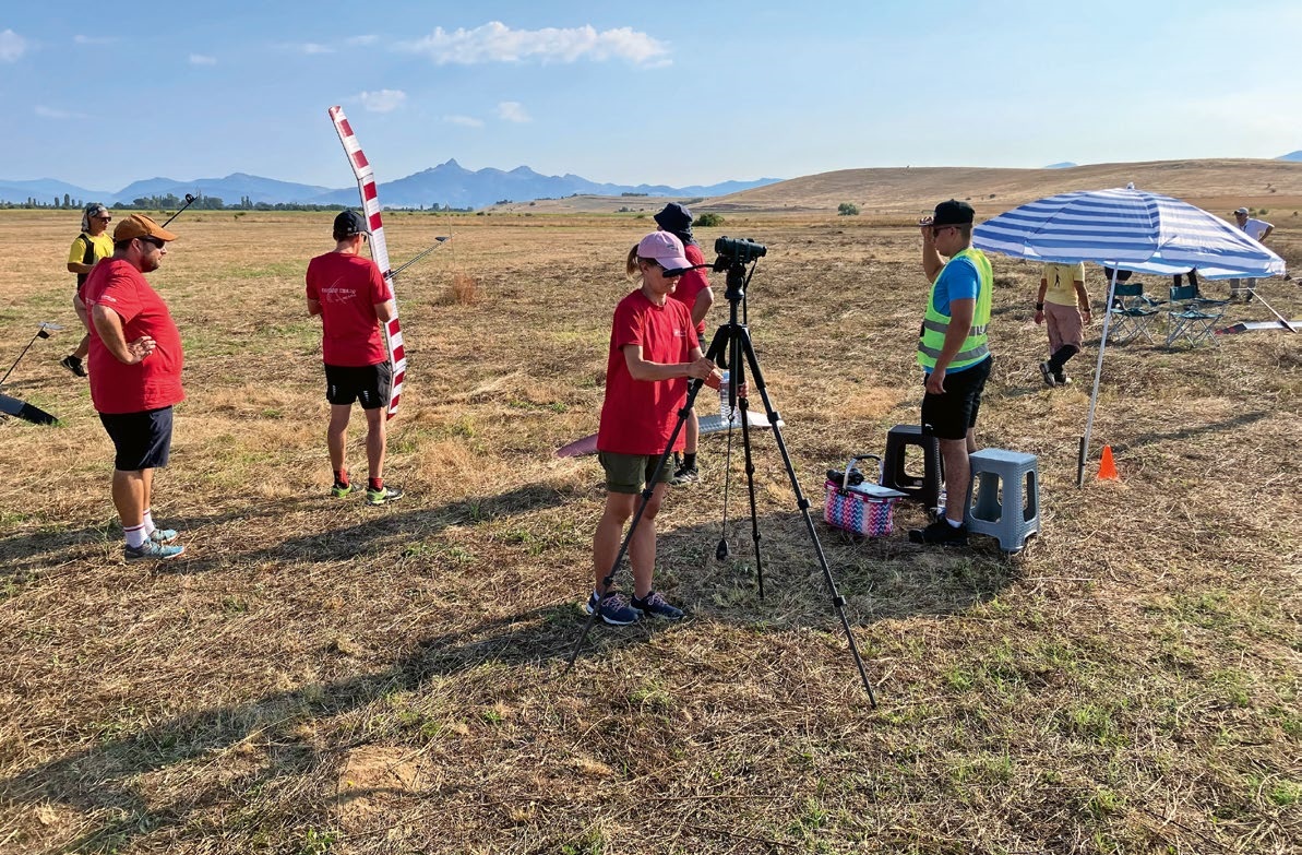
FREE FLIGHT IN THE MIDDLE OF SUMMER
Urs Muntwyler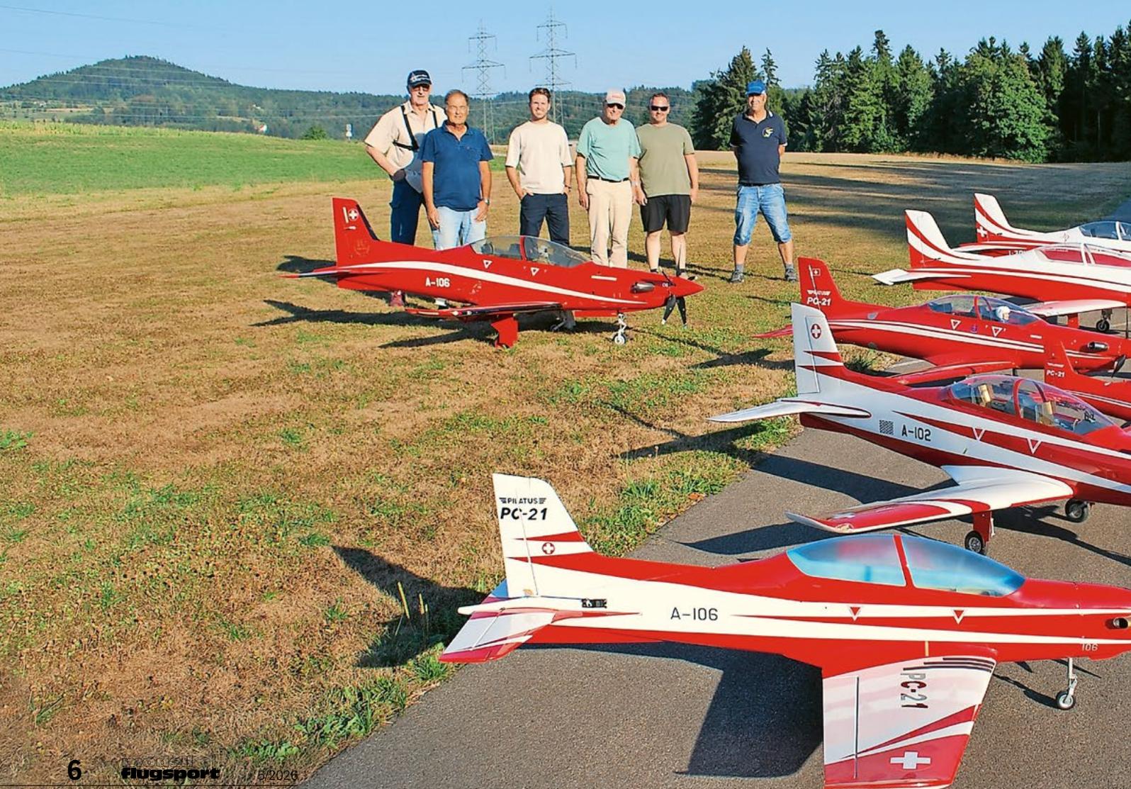
THE PC-21 STORY
Emil Giezendanner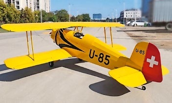
NEWS FROM HEBU
 Julia Bucher
FROM 0 TO 100
Markus Nussbaumer
MEMORIES
Wolfgang Völler
NOS REGION – A HUB FOR ELECTRIC AVIATION
Emil Giezendanner
Have you almost forgotten about aircraft that take off and land vertically?
Emil Giezendanner
DO YOU KNOW WHAT I MEAN IN THE LAND OF SMILES?
Emil Giezendanner