
Electric Aircraft Motors: Basics and Simple Measurements
In electric flight, only permanent-magnet DC motors are used. One of their advantages is that their operating behavior and the factors behind it are relatively easy to understand. It is also quite easy to predict operating conditions with good accuracy if a few key parameters describing the motor are known. Conversely, these parameters can be derived from simple measurements taken on the motor. The characteristics and possibilities will be presented below. To keep within the given scope, this must be done concisely. Less important details, lengthy derivations, etc., must necessarily be omitted.
To begin with, let's make two idealized simplifications that are generally accepted:
The rotating armature is subject to a frictional torque consisting of bearing, brush, and air friction. We assume that this frictional torque is constant, i.e., independent of the rotational speed.
The resulting error is minimal and has no practical significance.
The motor’s armature rotates in a magnetic field. If it contains iron (which is the case with a few exceptions in electric aircraft motors), harmful eddy currents are induced within it. In addition, the armature is remagnetized with each revolution, resulting in remagnetization (“hysteresis”) losses. Eddy current losses can be minimized through appropriate design (thin, insulated sheets = a sign of quality and suitability). Hysteresis losses are also kept low by using suitable, magnetically “soft” armature sheet metal. We therefore assume that eddy current and hysteresis losses are zero.
Experience shows that the resulting errors in the calculation results do not exceed 5% for good motors.
In motors with an ironless armature (bell-type armature, disc rotor), these losses do not occur at all, and the formulas apply exactly.
In the armature, the current flowing through the magnetic field generates a torque that is proportional to the current:
$$M_i = B \cdot I \quad (1)$$
$B$ is a constant determined by the motor’s design; it has the dimension $[Nm/A]$.
We will come back to this later. It is worth noting that neither rotational speed nor voltage, etc., appear in this formula. These factors naturally influence the current itself; however, when a current of magnitude $I$ flows, formula (1) holds. From this “internal” torque generated, we must subtract the friction torque to obtain the delivered, usable torque:
$$M = B \cdot I - M_R \quad (2)$$
As the armature winding rotates in the magnetic field, a voltage is induced in it; the motor acts simultaneously as a generator. This induced voltage is opposite in direction to the applied voltage and is therefore called back EMF.
The back-EMF is proportional to the rotational speed:
$$U_G = B' \cdot \omega \quad (3)$$
$\omega$ is the angular velocity of the armature; for this, the following applies
$$\omega = \frac{\eta \cdot n}{30} \quad (4)$$
( $n = 3.1416$ )
where $\eta$ = rotational speed $[U/min]$ . (For rough calculations, $\omega \approx 0.1 \cdot n$ )
$B'$ is (initially) again a design constant of the motor; it has the unit $[V·s]$.
It can now be proven that $B$ and $B'$ are the same; that is, $B = B'$. This can also be seen from the units, since
$1 [Nm/A] = 1 [Vsec]$; or $1 [Nm/sec] = 1 [VA] = 1 [Watt]$ (electromechanical equivalent)
Of course, this is not a proof; it merely shows that in the following formulas, it makes no difference whether we use the dimension $[Nm/A]$ or $[Vsec]$ for $B$; we simply choose whichever is more appropriate in each case.
From now on, we have only this one constant $B$; it is referred to as the generator constant or the torque constant of the motor.
The motor presents an electrical resistance to the current flowing through it. This resistance consists almost entirely of the resistance of the armature winding; in addition, there are smaller contributions from the
brushes, contact resistance between the brushes and the commutator, etc. Its value is $R [\Omega]$.
In itself, the resistance is also a design constant of the motor; unfortunately, this “constant” depends significantly on the motor temperature. As the temperature rises, so does the resistance; this causes the motor’s performance to deteriorate significantly. This can be calculated; however, we will omit that here and assume, for example, that we are always referring to the resistance at “operating temperature” (60–80 degrees housing temperature; up to twice that inside).
When taking measurements on the motor, this should always be done at the same temperature at which the motor operates in real-world conditions; otherwise, we’ll obtain unrealistically favorable values. Normally, therefore, let the motor warm up under load first!
In practical operation, it is advisable to cool the motor well for this reason alone; high motor temperatures reduce efficiency and waste energy.
The equivalent circuit for our motor consists of a generator connected in series with a resistor (Figure 1). We also need to account for the motor's inductance, which is also present
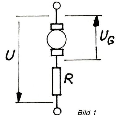
Figure 1
We do not need to take this into account here; however, it plays a major role in other applications (electronic speed controllers) and must not be neglected in those cases.
The operating voltage $U$ is applied to this series connection. Then the following applies
$$U - U_G = R \cdot I \quad (5)$$
(“driving” operating voltage – reverse voltage = remaining voltage across $R$; from this, the current $I$ follows)
$$U = U_G + R \cdot I \quad (6)$$
Substituting (3) into (6) yields
$$U = B \cdot \omega + R \cdot I \quad (7)$$
With Equations (7) and (2), we have found the two most important fundamental relationships for our motor. From these, we can derive everything else. The following quantities appear in these equations as constants specific to the motor:
$B$ = generator constant $[Nm/A]$ or $[Vsec]$
$R$ = motor resistance
$M_R$ = Friction torque $[N·m]$
It may seem surprising at first—but with these three quantities, the
motor is fully “described.” That is all we need to know—for now—to, for example, calculate an operating condition or to plot the motor diagrams.
In practice, however, there are additional factors to consider; for example, current values may result that are far too high in practice, or the heat loss may no longer be dissipated, etc.
Within the practically feasible, permissible operating range, these 3 constants provide all the basic data we need. Unfortunately, as a rule, these 3 parameters cannot be measured directly—or at least not easily and without significant measurement effort.
Later on, we’ll see how to determine them “indirectly” from simple measurements. For now, let’s assume that we already know $B$, $R$, and $M_R$.
It is useful to introduce a few characteristic parameters that, on the one hand, are more oriented toward practical considerations and, on the other hand, also aid in understanding and simplify calculations. These are:
- No-load speed $\omega_L$ or $n_L$
- No-load current $I_L$
- Short-circuit current $I_K$ (with the motor “stalled” and at rest)
- Short-circuit torque $M_K$ (“stall, stationary, or tipping torque”)
However, we must note here that—unlike the three constants mentioned above—we must specify the voltage at which $\eta_L$, $I_L$, $I_K$, and $M_K$ apply; we will see shortly that these values depend on the operating voltage.
First, we consider Eq. (7) and the case where $\omega = 0$ (stationary). Then
$$U = B \cdot 0 + R \cdot I_K$$
and the short-circuit current is
$$I_K = \frac{U}{R} \quad (8)$$
If we substitute $I_K$ for $I$ in Eq. (2), the short-circuit torque becomes
$$M_K = B \cdot I_K - M_R \quad (9)$$
Since $M_R \ll M_K$, it can be neglected in this special case, and we have
$$M_K \approx B \cdot I_K \quad (10)$$
Let us now consider the no-load condition: Here, the torque output is zero. From Eq. (2), we obtain
$$B \cdot I_L - M_R = 0$$
or, the no-load current $I_L = \frac{M_R}{B}$ (11)
Equation (7) can be solved for $\omega$ to give
$$\omega = \frac{U - R \cdot I}{B} \quad (12)$$
If we substitute the value found above for $I_L$, the no-load speed becomes
$$\omega_L = \frac{U}{B} - \frac{R \cdot M_R}{B^2} \quad (13)$$
or $n_L = \frac{30}{\pi} \left( \frac{U}{B} - \frac{R \cdot M_R}{B^2} \right)$ (14)
If we know $B$, $R$, and $M_R$, we can now use Eqs. (8) through (14) to calculate the parameters $n_L$, $I_L$, $I_K$, and $M_K$ for any voltage $U$.
From Eq. (11), we see that the no-load current becomes smaller as $M_R$ decreases and as $B$ increases. The no-load current is therefore a frequently used quality parameter; it captures two of the parameters at once.
Let’s now look at the variation of current, power, etc., across the entire operating range; these are known as characteristic curves. In professional engineering, it is common to plot all values as a function of the output torque. We will not use this method of representation here, but will instead plot the values against rotational speed. For our applications in model building, this is more intuitive and practical. Both methods of representation are, of course, equivalent, and they can easily be converted from one form to the other.
We can determine the current as a function of rotational speed from Eq. (7) by solving for $I$:
$$I = \frac{U}{R} - \frac{B \cdot \omega}{R} \quad (15)$$
Since $\frac{U}{R} = I_K$, we then have
$$I = I_K - \frac{B}{R} \cdot \omega \quad (16)$$
This is the equation of a straight line:
Starting from $I = I_K$ at $\omega = 0$, the current decreases uniformly to $I_L$ at $\omega_L$ (Figure 2).
We obtain the torque as a function of $\omega$ by substituting Eq. (15) into Eq. (2); this gives
$$M = \frac{B \cdot U}{R} - \frac{B^2}{R} \omega - M_R \quad (17)$$
Using Equations (8) and (9), this yields
$$M = M_K - \frac{B^2}{R} \cdot \omega \quad (18)$$
This, too, is an equation of a straight line; the torque decreases uniformly from its maximum value $M_K$ with increasing angular velocity until it reaches $M = 0$ at $\omega_L$ (Figure 3).
The output power is the product of torque and rotational speed. We obtain it by multiplying Eq. (18) by the rotational speed:
$$P_{OUT} = \omega \cdot M_K - \frac{B^2}{R} \omega^2 \quad (19)$$
This is the equation of a parabola; for $\omega = 0$ and $\omega = \omega_L$ , $P_{OUT} = 0$ ; between these points, there is a maximum (Figure 4).
We now want to know where the maximum lies and how large it is. The answer is obtained in the usual way by setting the derivative with respect to $\omega$ equal to zero; we will skip the calculation here and simply state the result:
$$\frac{\omega}{P_{max}} = \frac{1}{2} \frac{R \cdot M_K}{B^2} = \frac{1}{2} \omega_L \quad (20)$$
$$\text{and } P_{OUTmax} = \frac{1}{4} \frac{R \cdot M_K^2}{B^2} = \frac{1}{4} M_K \omega_L \quad (21)$$
For us in electric flight, only the RPM range above the maximum power—that is, above $\frac{1}{2} \omega_L$ —is of interest.
Below that, we would have to allow a much higher current to flow to maintain the same power; most of the supplied power would be “wasted” as heat in the process.
It is simply the product of voltage and current; using Eq. (17), we get
$$P_{IN} = U \cdot I = U \left( I_K - \frac{B}{R} \omega \right) \quad (22)$$
We observe a linear decrease from the maximum value $U \cdot I_K$ at steady state to $U \cdot I_L$ at $\omega_L$ (Figure 5).
Efficiency is the ratio of output power to input power, that is,
$$\eta = \frac{P_{OUT}}{P_{IN}} \quad (23)$$
We can substitute the expressions from Equations (19) and (22), which we derived earlier, into this equation to obtain
$$\eta = \frac{\omega (M_K - \frac{B^2}{R} \cdot \omega)}{U (I_K - \frac{B}{R} \cdot \omega)} \quad (24)$$
There is little benefit in trying to simplify this formula further; although the expression can be rearranged in various ways, it remains relatively complicated and confusing.
If we evaluate it point by point and plot it against $\omega$, we obtain a curve as shown in Figure 6. We are primarily interested in the magnitude of the maximum and the angular velocity at which it occurs.
We obtain this in the usual way from Eq. (24) by differentiating with respect to $\omega$ , setting the derivative to zero, and so on. We will skip this lengthy calculation here and look only at the result:
$$\frac{\omega}{\eta_{max}} = \frac{U}{B} \left( 1 - \sqrt{\frac{R \cdot M_R}{U \cdot B}} \right) \quad (25)$$
$$\text{and } \eta_{max} = \left( 1 - \sqrt{\frac{R \cdot M_R}{U \cdot B}} \right)^2 \quad (26)$$
If we substitute the expressions for $I_L$ and $I_K$ found earlier into Eqs. (25) and (26), we obtain the following simple formulas
$$\frac{\omega}{\eta_{max}} = \frac{U}{B} \left( 1 - \sqrt{\frac{I_L}{I_K}} \right) \quad (27)$$
$$\text{and } \eta_{max} = \left( 1 - \sqrt{\frac{I_L}{I_K}} \right)^2 \quad (28)$$
The smaller $I_L$ becomes and the larger $I_K$ becomes, the higher the maximum efficiency becomes and the higher the speed at which it is achieved. However, it does not make much sense to look only at a motor’s maximum efficiency; the higher it is, the closer it is to the no-load speed, the “sharper” the peak, the lower the power output at that point, and
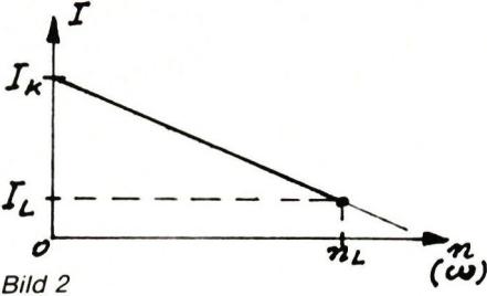
Image 2
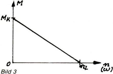
Figure 3
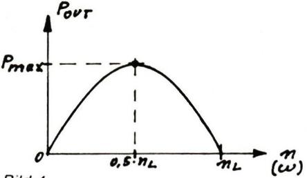
Figure 4
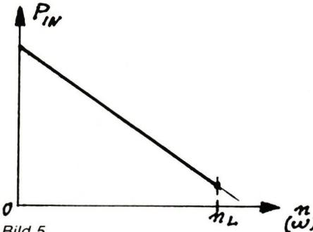
Figure 5
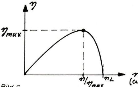
Figure 6
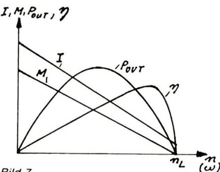
Figure 7
the more difficult it is in practice to maintain the corresponding speed. Instead, we should focus on how efficiency varies within a practically meaningful range—between the maximum power and maximum efficiency—and what value it has at the target power output. In practice, of course, the diagrams are not plotted individually, as we have done, but rather all the curves are plotted together on a single diagram (Figure 7). Which operating point—that is, which rotational speed—is selected depends entirely on the specific application; e.g., on the model type and characteristics, the propeller, any gearbox, the flight mission, etc. The formulas provided, as well as the engine characteristic curves, are always essential foundations in this context.
We have seen previously that we can perform all the calculations for our motor as long as we know the motor parameters B, R, and MR. We can only obtain these from the manufacturer’s documentation in special cases. We must therefore determine them ourselves. This can be done by taking measurements on the motor; or—if available—by analyzing the data and/or diagrams provided by the manufacturer. We’ll set the latter aside for now; we’ll come back to it later. The problem is that we cannot measure B, R, and MR using simple methods, or can only do so with very low accuracy. For example, in a typical electric aircraft motor, R is only a fraction of an ohm, which is no longer measurable with simple measuring instruments. Or, what model builder actually has equipment for accurately measuring torque?
We must therefore try to reduce and limit the measurements to easily measurable quantities; these include, for example, voltage, current, and rotational speed. We will then see how we can calculate our parameters from these values. The method used is little known among model builders—quite unjustly so, since it is easy to apply. We don’t need a “proper” test bench at all; just a good voltmeter and ammeter, as well as an accurate tachometer. These instruments can be purchased today at a relatively low cost with the required accuracy; often, they’re already available in the model-building workshop anyway. The measuring instruments should have an accuracy of 2% or better if possible; with digital measuring instruments, this requirement is usually easy to meet. Nevertheless, we must expect an error of about ±10% in our calculated values due to factors such as fluctuating motor resistance, unfavorable error propagation in some cases, idealization, etc. For our application in model aviation, where the
final fine-tuning must be done in practice for other reasons anyway, this level of accuracy in the calculated values is sufficient.
The measurement setup is shown in Figure 8. Ideally, a power supply with an adjustable output voltage and the required current capacity can serve as the current source. However, the same results can be achieved—albeit with less convenience—using the model’s existing flight batteries; in extreme cases, the entire measurement can even be performed with the motor installed in the model.
As shown in Figure 8, note that the voltmeter must be connected behind the ammeter—that is, directly to the motor terminals; otherwise, a significant, load-dependent measurement error may occur due to the voltage drop across the ammeter.
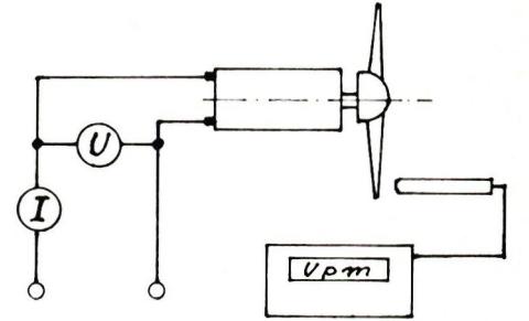
Figure 8
Let’s assume that we have connected a load (propeller) to the motor and that it is running at the terminal voltage U. We now measure the current consumption I and the rotational speed n. We don’t need to know anything else about the load itself! We label the values of U, I, and n that we have just measured with the subscript “1.” Then, of course, our formula (7) from above applies:
$$U_1 = B \cdot \omega_1 + R \cdot I_1 \quad (29)$$
Now we mount a different propeller on the motor and take another measurement. We obtain different values for I and n; possibly also for U. These values are designated with the index “2.” Then the following applies again:
$$U_2 = B \cdot \omega_2 + R \cdot I_2 \quad (30)$$
With Equations (29) and (30), we now have two equations for the two unknowns B and R. Using standard methods, we can derive the determining equations for B and R; we will omit this brief intermediate calculation here. The result is:
$$B = \frac{U_1 \cdot I_2 - U_2 \cdot I_1}{I_2 \cdot \omega_1 - I_1 \cdot \omega_2} \quad (31)$$
$$R = \frac{U_2 \cdot \omega_1 - U_1 \cdot \omega_2}{I_2 \cdot \omega_1 - I_1 \cdot \omega_2} \quad (32)$$
To determine MR, we now need to measure the no-load current IL; using equation (11), which we solve for MR, we obtain:
$$M_R = B \cdot I_L \quad (33)$$
We have already found the generator constant B, which we need for this, using Eq. (31).
The following must be noted when performing these measurements:
- The two measurements should be taken at rotational speeds (or currents) that differ as much as possible from one another, so that measurement errors do not have significant consequences. For example, for the first measurement, we choose the smallest possible propeller so that the rotational speed is high (close to idle); for the second measurement, we then choose a large propeller that gives us a rotational speed, for example, close to half the idle speed.
- Caution: It is possible that the motor must not be operated at idle at its rated voltage, because otherwise the armature would “fly apart.” If necessary, therefore, reduce the operating voltage during high-speed measurements.
- Of course, we can take more than just two measurements; for example, using several different available propellers. The values calculated from these measurements will vary due to unavoidable measurement errors; we can then take the average. If differences greater than approximately $\pm 10\%$ occur, there is likely a measurement or calculation error. By comparing individual terms, calculating auxiliary values (e.g., $I_K$ , $M_K$), or by plotting the measurement points on the graphs (at constant voltage, the points must align with the curves discussed), conclusions can be drawn about the value that is likely to be incorrect.
- In the above formulas, $\omega$ must be substituted; we obtain $\omega$ from the measured rotational speed $n$ by multiplying by 0.1047; see also Eq. (4).
Now that we have learned the procedure for determining the parameters from measurements, it is actually already clear how to proceed if we do not take any measurements at all but instead want to use the diagrams provided by the manufacturer. From the diagrams, we can immediately determine $I$ and $n$ for two points that are far apart, as well as the no-load speed. The voltage for which the diagram applies is always specified on the diagram itself. It is particularly simple if we choose the no-load condition as one of the two points right away. However, it is always preferable to take your own precise measurement, since this applies specifically to the motor in question, whereas the diagram normally only shows typical values from which the motor in question may deviate due to manufacturing tolerances.
Motor: Mabuchi 550 Measurement
1: 6"×4" propeller;
$U_1 = 6.0\text{ V}$ ; $I_1 = 3.8\text{ A}$ ; $n_1 = 8050\text{ rpm}$
Measurement 2: 9"×4" propeller;
$U_2 = 6.0\text{ V}$ ; $I_2 = 7.8\text{ A}$ ; $n_2 = 6950\text{ rpm}$
First,
$\omega_1 = 0.1047 \cdot 8050 = 843\text{ sec}^{-1}$ ;
$\omega_2 = 0.1047 \cdot 6950 = 728\text{ sec}^{-1}$ .
Thus,
$$B = \frac{U_1 \cdot I_2 - U_2 \cdot I_1}{I_2 \cdot \omega_1 - I_1 \cdot \omega_2} = \frac{6 \cdot 7.8 - 6 \cdot 3.8}{7.8 \cdot 843 - 3.8 \cdot 728} = 0.0063\text{ Nm/A}.$$
and
$$R = \frac{U_2 \cdot \omega_1 - U_1 \cdot \omega_2}{I_2 \cdot \omega_1 - I_1 \cdot \omega_2} = \frac{6 \cdot 843 - 6 \cdot 728}{7.8 \cdot 843 - 3.8 \cdot 728} = 0.18\Omega.$$
Furthermore, the following was measured:
$$I_L = 0.7\text{ A at } 6.0\text{ V};$$
$$\text{so that } M_R = B \cdot I_L = 0.0063 \cdot 0.7 = 0.0044\text{ Nm}.$$
At $U = 6\text{ V}$, the following is also calculated:
$$I_K = \frac{U}{R} = \frac{6}{0.18} = 33.3\text{ A};$$
$$M_K = B \cdot I_K - M_R = 0.0063 \cdot 33.3 - 0.0044 = 0.205\text{ Nm}$$
$$\text{and } \eta_{max} = \left(1 - \sqrt{\frac{I_L}{I_K}}\right)^2 = \left(1 - \sqrt{\frac{0.7}{33.3}}\right)^2 = 0.73\text{ (73\%)}$$
where
$$\omega_{\eta_{max}} = \frac{U}{B} \left(1 - \sqrt{\frac{I_L}{I_K}}\right) = \frac{6}{0.0063} \left(1 - \sqrt{\frac{0.7}{33.3}}\right) = 819\text{ sec}^{-1}$$
$$= \frac{30}{n} \cdot 819 = 7.820\text{ rpm}$$
No-load speed
$$\omega_L = \frac{U}{B} - \frac{R \cdot M_R}{B^2} = \frac{6}{0.0063} - \frac{0.18 \cdot 0.0044}{0.0063^2} = 952\text{ sec}^{-1}; \quad n_L = 9.094\text{ rpm}$$
The speed range for our applications is therefore approximately between 5,000 and 7,500 rpm (at 6 volts!).
With the values we've found for $B$, $R$, and $M_R$, we can do much more than just get an idea of the motor's characteristics in this particular case.
Electric motors are very “flexible” drives that—at least for short periods—can handle significant overloads. Therefore, it is often of interest to know what happens, for example, when the operating voltage is increased. With the formulas provided here, this is no problem. We know the motor parameters $B$, $R$, and $M_R$ from measurements and calculations; we simply need to substitute the new voltage $U$ into the formulas to obtain all the relevant data. In addition, we can, of course, plot the complete characteristic curves for the new voltage.
If we know from experience the maximum power dissipation (input power $P_{IN}$ – output power $P_{OUT}$ ) that is permissible for our motor in a specific installation scenario, we can determine from the new characteristic curve diagram the minimum speed at which the motor must operate at the increased voltage so that the (unchanged) power dissipation is not exceeded.
By determining the parameters, we have, so to speak, “calibrated” our motor. This allows us, for example, to use Eq. (2) to measure the required propeller torque at a given rotational speed. All we need to do is measure the motor’s current consumption! We substitute the measured value $I$ and the known data $B$ and $M_R$ into Eq. (2) to obtain the torque delivered by the motor.
If we also measure the rotational speed at the same time, we can determine the power absorbed by the propeller:
$$\text{We have } P_{Prop} = P_{OUT} = M \cdot \omega \quad (34)$$
##### Example:
Motor, motor parameters as in the previous example; TF Nylon 8"×4" propeller
;
measured $U = 8\text{ V}$ ; $I = 9.2\text{ A}$ ; $n = 8850\text{ rpm}$
We have
$$\omega = 0.1047 \cdot 8850 = 927\text{ sec}^{-1}$$
$$M = B \cdot I - M_R = 0.0063 \cdot 9.2 - 0.0044 = 0.053\text{ Nm}$$
$$P_{OUT} = M \cdot \omega = 0.053 \cdot 927 = 49.1\text{ W}$$
$$\text{On the other hand, } P_{IN} = U \cdot I = 8 \cdot 9.2 = 73.6\text{ W}$$
thus, at the operating point
$$\eta = \frac{P_{OUT}}{P_{IN}} = \frac{49.1}{73.6} = 0.67$$
In this way, we can obtain valuable data about our propulsion system. However, we will only briefly touch on these possibilities here, since a more in-depth analysis would also require elements of propeller calculation, the presentation of which would go beyond the scope of this discussion.
Based on these fundamentals, a method is derived that allows basic motor data to be determined through simple measurements on standard electric aircraft motors.
Using these values, it is possible to calculate the motor’s characteristic curves, key parameters, and so on; this provides a comprehensive understanding of the motor’s properties. With the motor data, it is then also possible to draw conclusions about the loads driven by the motor using simple measurements.
This presentation was given by Dipl. Ing. Helmut Schenk at the 3rd Swiss Electric Flight Symposium in 1983 at Technorama Winterthur.


News from HEBU
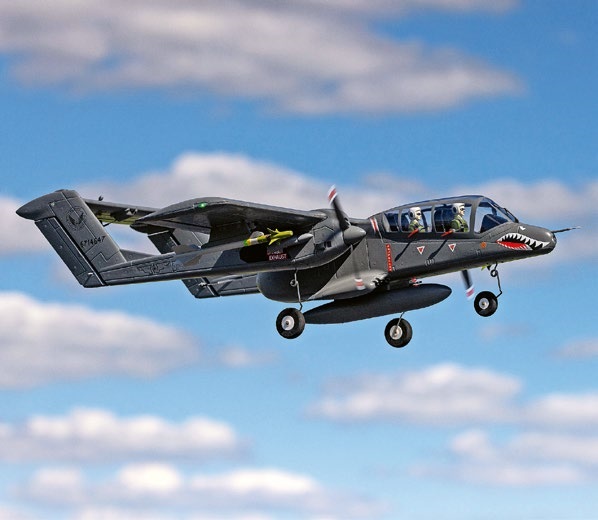
HORIZON HOBBY/LEMACO NEWS: MICRO OV-10 BRONCO 645 MM BY E-FLITE

PRIDE AND GOOD IDEAS
 Markus Nussbaumer

TEAM MANAGER "THIS" BOSSHARD
 Rodito Nussbaumer

YOU KNOW WHAT I MEAN? 125 YEARS OF THE SWISS AERO CLUB
 Emil Giezendanner

F3A EUROPEAN CHAMPIONSHIPS IN ST-MACAIRE, FRANCE
 Matthias Bosshard
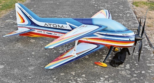
ATOM, THE NEW DOUBLE-DECKER FROM CPLR
Matthias Bosshard
SUMMER FUN 2026 AT MG USTER
Martin Wunderli
What's New at Leomotion.com
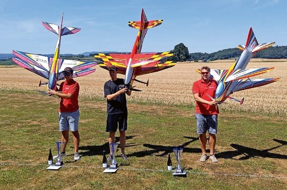
52. 2026 ALPS CUP
Emil Giezendanner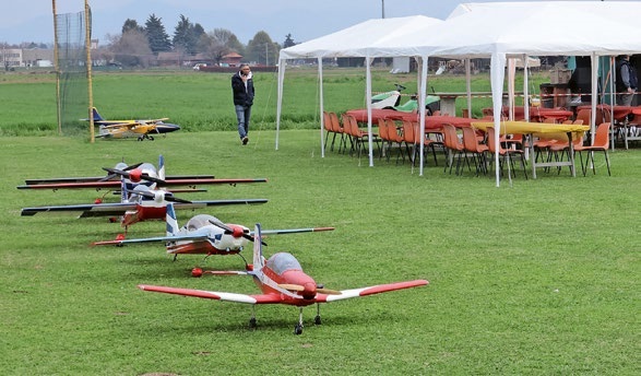
TWIN TOWN PARTNERSHIP
Wolfgang Voeller
34th HAHNENMOOS ALPINE MODEL AIRPLANE CAMP
Res Dauwalder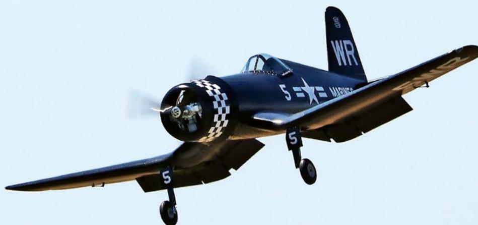
CORSAIR F4U – A WARBIRD WITH A MEMORABLE LOOK
Jürgen Rosenberger, Jürgen Prinz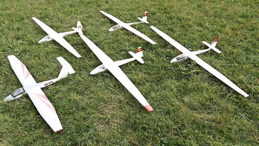
SMALL, MODEL-LIKE SAILBOATS
Res Dauwalder
TRY-OUT DAY AT MFV WETTINGEN
Urs Keller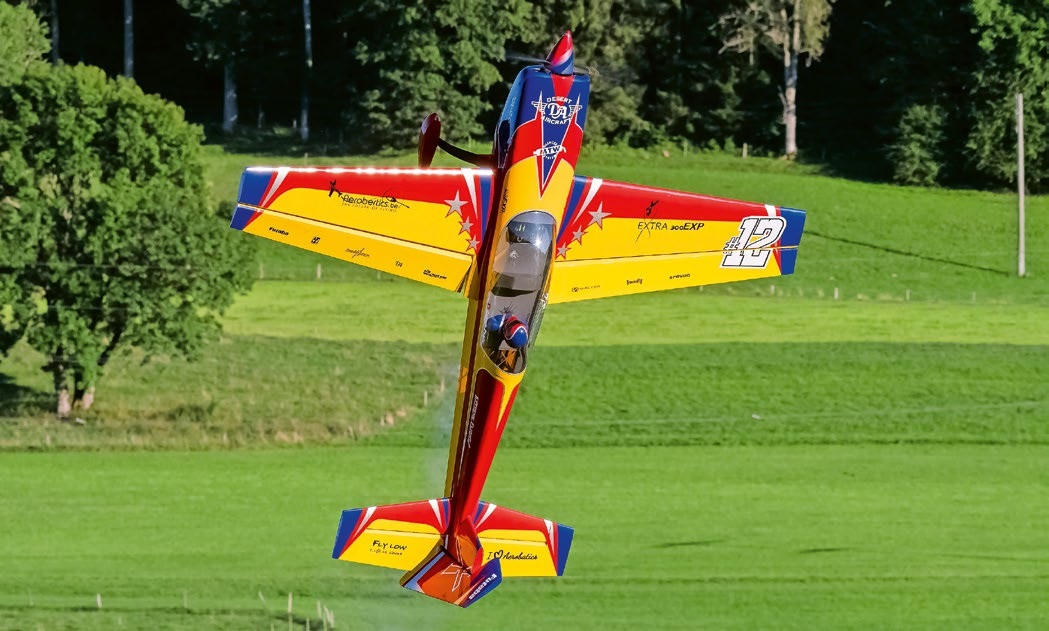
WELCOME, NEW MEMBER!
Andrea Bolliger
FREE FLIGHT IN THE MIDDLE OF SUMMER
Urs Muntwyler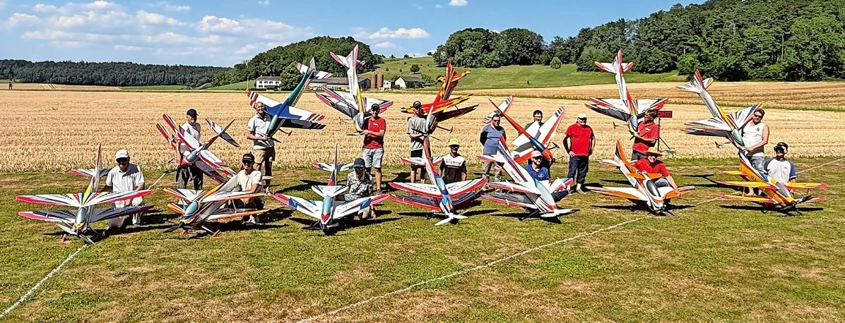
COUPE DES ALPES – OBSERVE AND LEARN
Rodito Nussbaumer
EURO CONTEST GLIDER ACRO TOUR AUSTRIA 2026
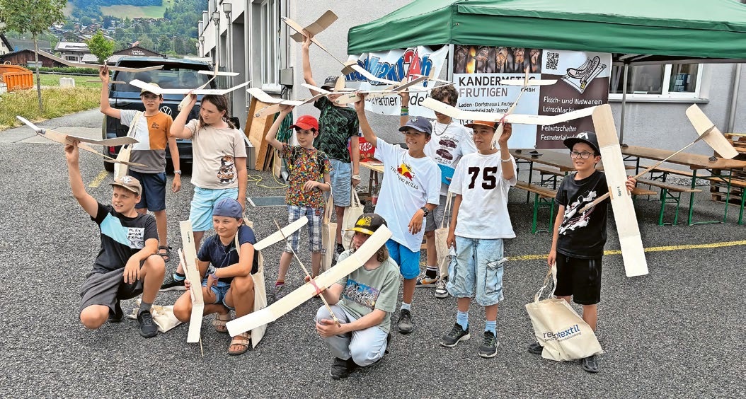
BY YOUTH, FOR YOUTH
Lorena Betschen
INSIGHTS INTO THE HISTORY OF SEAPLANES
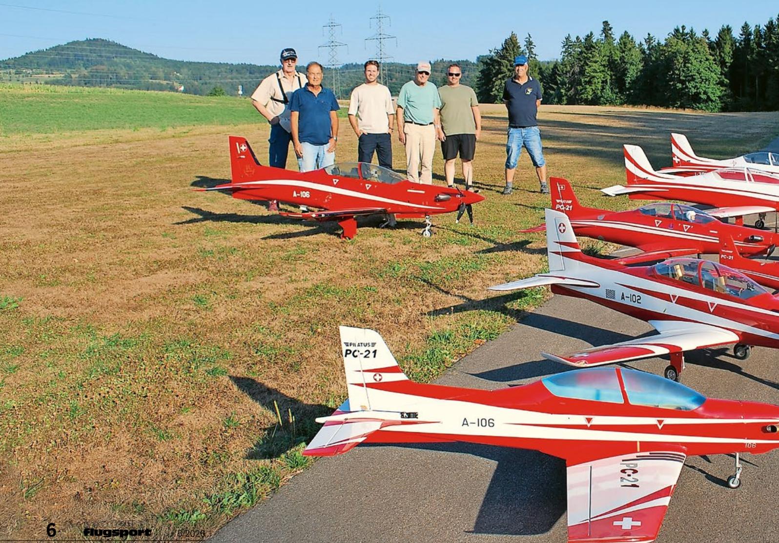
THE PC-21 STORY
Emil Giezendanner
NEWS FROM HEBU
 Julia Bucher
FROM 0 TO 100
Markus Nussbaumer
MEMORIES
Wolfgang Völler
NOS REGION – A HUB FOR ELECTRIC AVIATION
Emil Giezendanner
DO YOU KNOW WHAT I MEAN IN THE LAND OF SMILES?
Emil Giezendanner
Have you almost forgotten about aircraft that take off and land vertically?
Emil Giezendanner