
F3B Glider Models – Comparison of the Aerodynamic Properties of Model Aircraft Airfoils
The F3B Series A competition class essentially requires the following of glider models:
- low sink rate for sustained flight,
- a good glide ratio at moderate airspeed for distance flight,
- a good glide ratio at high airspeed for speed flight.
When designing a glider for this category, a compromise must be found between these diverse requirements, while also taking into account other factors such as high-launch characteristics, stall behavior, turning performance, and so on.
The question of the best airfoil has long been a source of heated debate among model builders. Due to a lack of precise knowledge and documentation, it usually comes down to one claim pitted against another. In the following, we will address the problem of how to establish an objective basis for selecting airfoils for F3B models. To do this, we will not delve into laborious flight performance calculations or complicated optimization questions, but rather determine simple key figures from the available aerodynamic data that allow for a quick comparison between different airfoils.
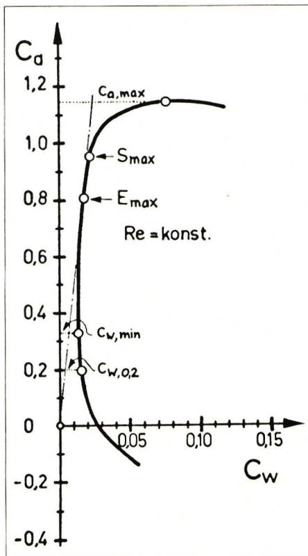
The aerodynamic properties of airfoils with respect to lift and drag, as determined from experiments and calculations, are usually plotted on polar diagrams. Fig. 1 schematically shows the airfoil polar (lift coefficient $c_a$ as a function of the drag coefficient $c_w$ ) of an airfoil suitable for RC gliding. As is well known, the shape and position of these curves depend not only on the airfoil contour but also on the Reynolds number $Re$ , which can be calculated approximately using the rule of thumb $Re = 70 \cdot v \cdot t$ . The airspeed $v$ should be entered in m/s and the airfoil depth $t$ in mm. An estimate shows that for F3B models, the Reynolds numbers on the wing range roughly from $Re = 50,000$ (slow flight, wingtip, low wing loading) and $Re = 500,000$ (maximum speed, wing root, high wing loading).
Airfoil polars at a constant Reynolds number are of limited use for a direct comparison of airfoils. To clearly characterize the aerodynamic properties, we therefore use several key parameters derived from the airfoil polars (the corresponding theory can be found in the book by F. W. Schmitz [1]):
Maximum airfoil glide ratio $E_{max} = (c_a/c_w)_{max}$ (In the literature, the reciprocal $c_w/c_a$ is often referred to as the glide ratio.) $E_{max}$ characterizes a profile in terms of the achievable glide angle; that is, the larger the glide ratio, the better the achievable glide angle. The maximum glide ratio can be easily determined by drawing a tangent to the polar curve starting from the origin; see Fig. 1. $E_{max}$ is decisive at moderate flight speeds, i.e., in the range $Re = 100,000 \dots 200,000$.
Maximum profile sink rate $S_{max} = (c_a^{1.5}/c_w)_{max}$ (In the literature, the quantity $c_w^2/c_a^3$ is often referred to as the climb rate or sink rate.) $S_{max}$ characterizes an airfoil in terms of the achievable minimum sink rate; that is, the larger the sink rate, the smaller the achievable minimum sink rate. The sink rate is decisive during slow flight, i.e., in the range $Re = 50,000 \dots 150,000$.
Airfoil drag coefficient $c_{w,0,2}$ Even in high-speed flight—that is, at low lift coefficients—the F3B model must fly with a good glide angle. In this regard, a wing profile is characterized by the drag coefficient $c_{w,0,2}$ at a lift coefficient of $c_a = 0.2$ . The smaller $c_{w,0,2}$ is, the better the high-speed flight performance that can be achieved. The value $c_a = 0.2$ is arbitrarily defined; for a model with a wing loading of $35 \text{ g/dm}^2$, it corresponds to an airspeed of approximately $17 \text{ m/s}$. The relevant range for this parameter is $Re = 200,000 \dots 400,000$.
It should be noted that during high-speed flight, the lift coefficient can be less than $0.1$. To achieve outstanding high-speed flight performance, the profile drag must therefore remain low, down to approximately $c_a = 0$.
Maximum profile lift coefficient $c_{a,max}$ $c_{a,max}$ characterizes a profile in terms of the lowest achievable flight speed; that is, the larger the maximum profile lift coefficient, the lower the lowest achievable flight speed. The maximum airfoil lift coefficient is particularly important for tight circling in thermals and for high-altitude takeoffs. The relevant range is $Re = 50000 \dots 100000$.
Minimum airfoil drag coefficient $c_{w,min}$ The significance of $c_{w,min}$ is somewhat less than that of the parameters already discussed when selecting airfoils for F3B models. $c_{w,min}$ can be regarded as a measure of a profile’s “aerodynamic quality.”
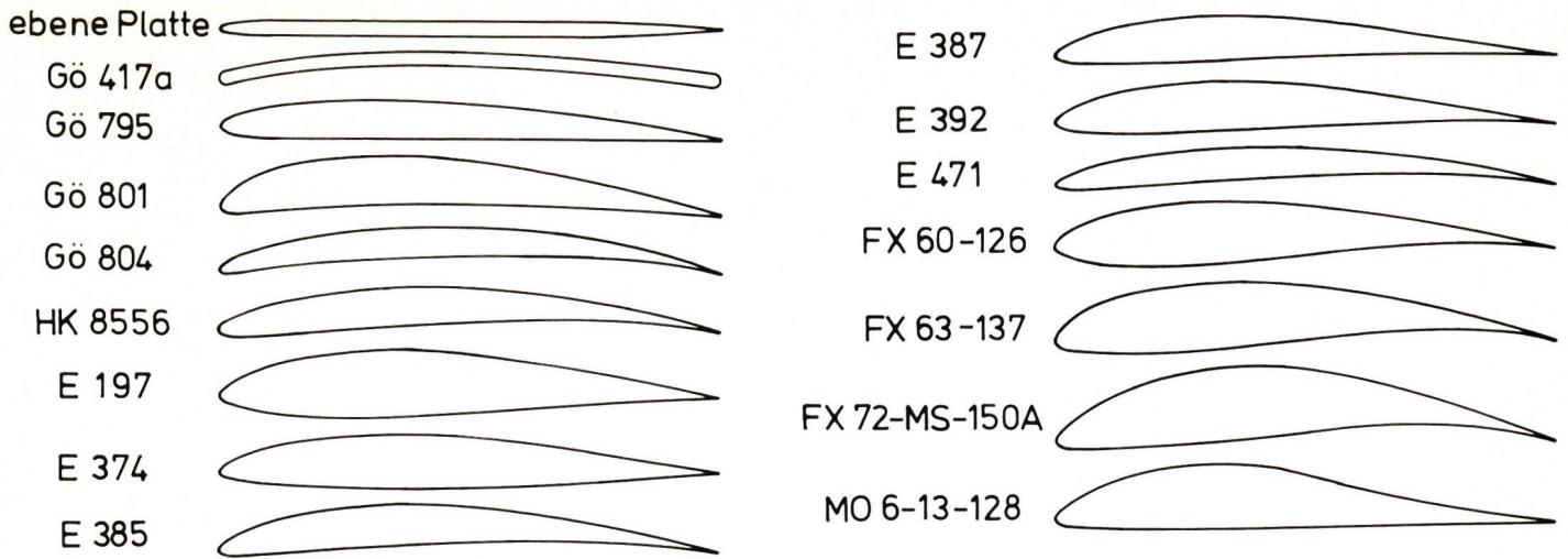
For 16 airfoils for which measured or calculated polars are known at Reynolds numbers less than $10^6$—see the bibliography at the end—the performance metrics discussed in the previous section were determined. The airfoils examined are summarized in Fig. 2. As can already be seen from the profile contours, only a portion of the selected profiles is suitable for the wings of F3B gliders. The rest were included in the comparison to illustrate the limits of what is currently achievable. Table 1 provides an overview of the best values for the various performance metrics. When evaluating these values, it should be noted that, of course, the same profile cannot simultaneously yield the largest $S_{max}$ and the smallest $c_{w0,2}$. Table 1 clearly illustrates how much the best values of the aerodynamic parameters improve as the Reynolds number increases. For this reason, the larger glider is always superior to the smaller one in terms of aerodynamics. Noteworthy is the striking difference between measured and calculated values in the relevant range of the Reynolds number. It is hoped that new experiments being conducted by Prof. Wortmann in Stuttgart will shed light on this issue.
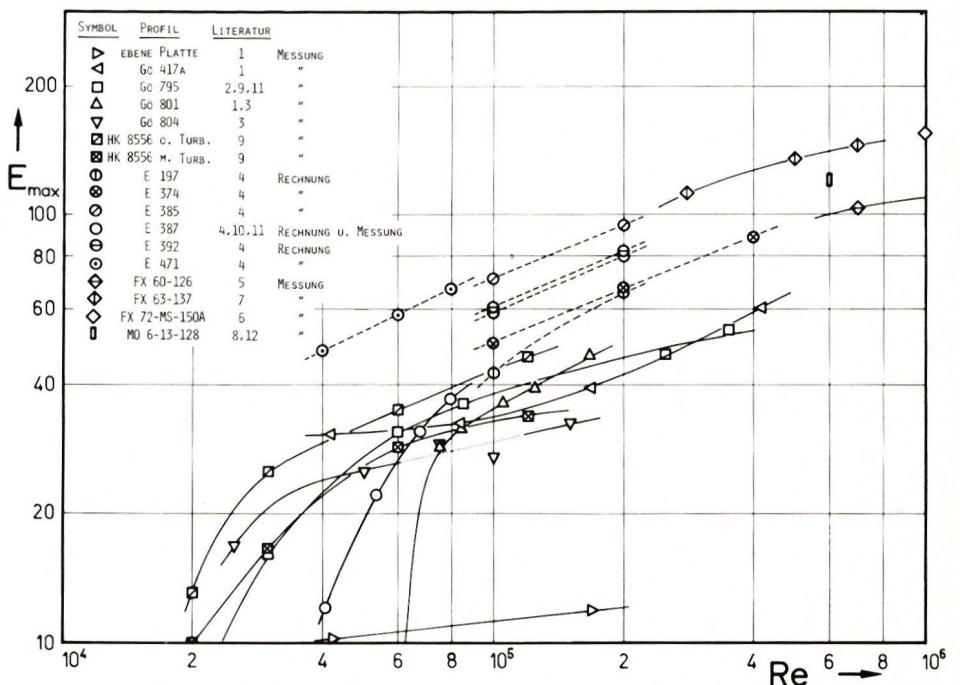
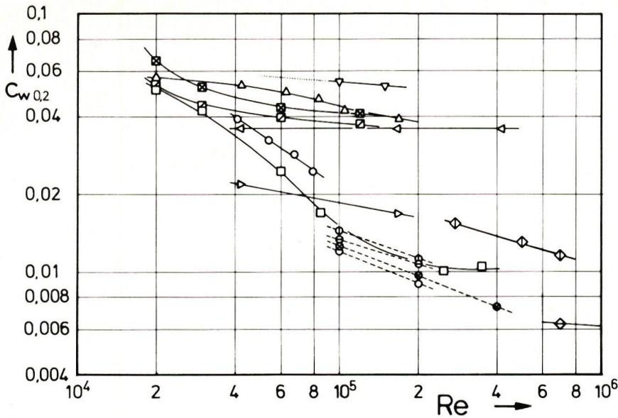
In Figures 3 through 7, $E_{max}$ , $S_{max}$ , $c_{w,0,2}$ , $c_{a\;max}$, and $c_{w\;min}$ are plotted as functions of the Reynolds number, insofar as these quantities could be determined at all from the available documentation. For example, in Fig. 6, data for $c_{a\;max}$ of the Eppler profiles—with the exception of E 387—are missing, since the maximum lift can only be estimated from the calculated polars in [4]. Measured values are connected by solid lines, while calculated values are connected by dashed lines. As already noted for the best values of the various profiles in Table 1, Figures 3 through 7 also show that the aerodynamic characteristics of individual profiles generally improve with increasing Reynolds number. Clearly visible is the drastic deterioration in the aerodynamic properties of most profiles at Reynolds numbers less than 100,000, which is linked to the phenomenon of the critical Reynolds number; see [1].
Table 2 compiles the characteristics of the individual airfoils at a typical Reynolds number for each, to allow for a direct comparison. The figures are derived in part from the curves in Figures 3 through 6, in part extrapolated from these curves, and in part estimated. An assessment of their suitability as airfoil profiles for F3B competition gliders is provided in Table 2.
| Reynolds number | 20,000 | 50,000 | 100,000 | 500,000 | 1,000,000 | |
|---|---|---|---|---|---|---|
| $E_{max}$ | Measurement | 13 | 32 | 43 | 135 | 155 |
| Invoice | - | 53 | 71 | - | - | |
| $S_{max}$ | Measurement | 17 | 35 | 44 | 170 | 210 |
| Invoice | - | 58 | 81 | - | - | |
| $c_{w\;0.2}$ | Measurement | 0.051 | 0.022 | 0.016 | - | 0.006 |
| Calculation | - | - | 0.012 | 0.007 | - | |
| $c_{a\;max}$ | Measurement | 1.2 | 1.3 | 1.4 | 1.8 | 1.9 |
| $c_{w\;min}$ | Measurement | 0.036 | 0.013 | 0.011 | 0.007 | 0.006 |
Table 1: Best values for the key metrics of 16 profiles
The comparison methodology described in the second and third sections allows for a quick assessment of a profile’s suitability. The various performance metrics immediately reveal in which characteristics a profile is superior or inferior to other profiles.
One occasionally hears and reads about the use of competition models equipped with flaps or similar systems. It is conceivable that such aerodynamic refinements, similar to those found in gliders, will also become standard in F3B models. There is currently no aerodynamic literature on the optimal design and effectiveness of flap profiles in the field of RC gliding. This leaves model builders with a wide field of opportunity to bring their own ideas to life.
| Profile | $E_{max}$ Re=125,000 | $S_{max}$ Re=100,000 | $c_w$ 0.2 Re=250,000 | $c_a$ max Re=75,000 | Suitability for F3B | Notes : M = measurement, R = calculation |
|---|---|---|---|---|---|---|
| flat plate | 11 | 7 | (0.016) | 0.53 | - | M, for tail surfaces |
| Gö 417a | 36 | 33 | 0.036 | 1.09 | - | M, for smaller Re numbers |
| Gö 795 | 41 | 33 | 0.010 | 0.69 | + | M, $c_a$ max small (low curvature) |
| Gö 801 | 40 | 38 | (0.038) | 1.36 | o | M, poor high-speed flight |
| Gö 804 | 30 | 30 | (0.050) | 1.31 | - | M, designed for F1A |
| HK 8556 | 47 | 44 | (0.035?) | 1.23 | - | M, " " " |
| HK 8556 with turbo | 34 | 33 | (0.038?) | 1.21 | - | M, " " " |
| E 197 | 50 | 39 | 0.0105 | (1.0?) | o | R, for large sailboats |
| E 374 | 55 | 47 | 0.0088 | (1.0?) | o | R, very good for acro pilots |
| E 385 | 78 | 81 | ... (>) | (1.4?) | o | R, excellent thermals |
| E 387 | 65(45?M) | 60 (42?M) | 0.0082 R | 1.23 M | ++ | R, M, and extrapolated from measurement |
| E 392 | 67 | 64 | 0.0098 | (1.2?) | ++ | R, high-speed flight slightly less favorable |
| E 471 | (84?) | (80) | ... (>) | (1.3?) | - | R, designed for F1A |
| FX 60-126 | ... | ... | (0.008?) | ... | ? | M, calculated for gliders |
| FX 63-137 | ... | ... | 0.016 | ... | ? | M, calculated for human-powered aircraft |
| FX 72-MS-150A | ... | ... | ... | ... | - | M, " " " " " |
| MO 6-13-128 | ... | ... | ... | ... | ? | M, calculated for Re=600,000 |
Table 2 (The following profiles from the Eppler series are also well suited for F3B models but were not included in the comparison: E 193 / E 176 / E 178; see [4]).
Explanation of symbols:
| ( ) extrapolated value | - unsuitable |
| ? estimated value, uncertain | ○ usable |
| ... cannot be determined from the documentation | + good |
| > large | ++ very good |
| ? questionable |
[1] F. W. Schmitz: Aerodynamics of Model Aircraft, 6th ed. Luftfahrt-Verlag Walter Zuerl, D-8031 Steinebach-Wörthsee.
[2] G. Muesmann: Measurements and Boundary Layer Observations on Affinely Thickened Blower Profiles as a Function of the Reynolds Number. Journal of Aeronautical Sciences 7 (1959), No. 9, pp. 253–264.
[3] K. Kraemer: Airfoil Profiles in the Critical Reynolds Number Range. Engineering Research 27 (1961), pp. 33–46.
[4] W. Thies: Eppler Profiles 1 and 2. Verlag für Technik und Handwerk, A. u. B. Ledertheil, 757 Baden-Baden.
[5] F. X. Wortmann: Some Laminar Profiles for Gliders. Aero-Revue (1963), No. 11, pp. 647–651.
[6] F. X. Wortmann: Airfoils with a high lift-to-drag ratio at a Reynolds number of about one million. Motorless Flight Research 1972. NASA CR-2315 (Nov. 1973).
[7] D. Althaus: Stuttgart Airfoil Catalog I. Institute for Aerodynamics and Gas Dynamics at the University of Stuttgart, 1972.
[8] S. J. Miley: An analysis of the design of airfoil sections for low Reynolds numbers. State College, Mississippi (USA), 1972.
[9] B. Horeni, J. Lnenicka: Aerodynamics for Model Makers. Modelár (1974), Issues 4, 5, and 6.
[10] W. H. Phillips: Low-speed wind-tunnel tests of two airfoils suitable for models. Report of the Ninth Annual Symposium of the National Free Flight Society for 1976 (USA).
[11] R. Girsberger: Results of wind tunnel measurements on model airfoils. Aero-Revue 1977, No. 12, pp. 737–741.
[12] R. Girsberger: Modern Airfoils—What’s Behind Them? Modell-Flugsport (1977), Issues 5 and 6.
With a wry smile, the author of the *Profil* article series told us that his work at MFS had already been featured in *Nebelspalter*. Ed.
This aerodynamic body shape is optimally molded by the sports physician while the infant's bones are still soft. (From "Nebelspalter")

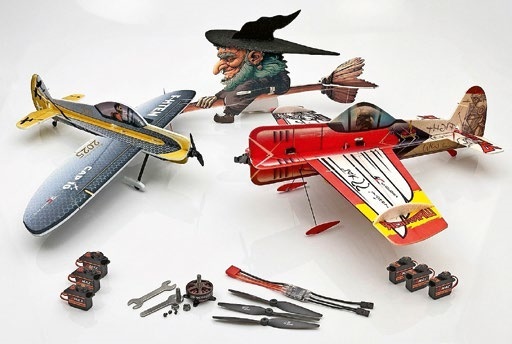
News from HEBU
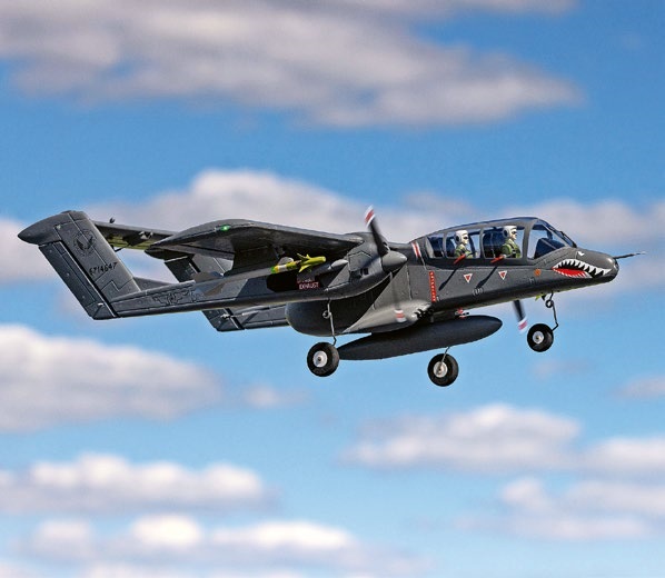
HORIZON HOBBY/LEMACO NEWS: MICRO OV-10 BRONCO 645 MM BY E-FLITE

PRIDE AND GOOD IDEAS
 Markus Nussbaumer
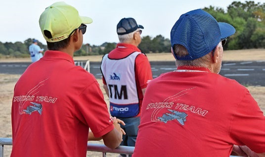
TEAM MANAGER "THIS" BOSSHARD
 Rodito Nussbaumer
YOU KNOW WHAT I MEAN? 125 YEARS OF THE SWISS AERO CLUB
 Emil Giezendanner
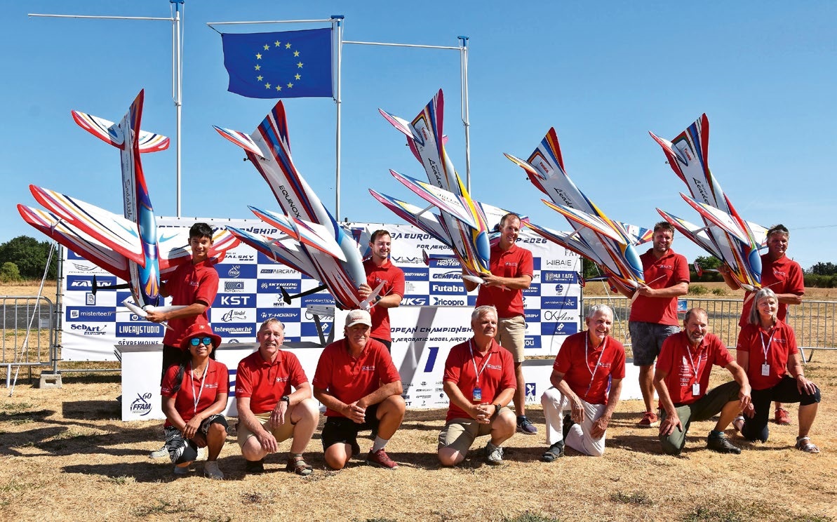
F3A EUROPEAN CHAMPIONSHIPS IN ST-MACAIRE, FRANCE
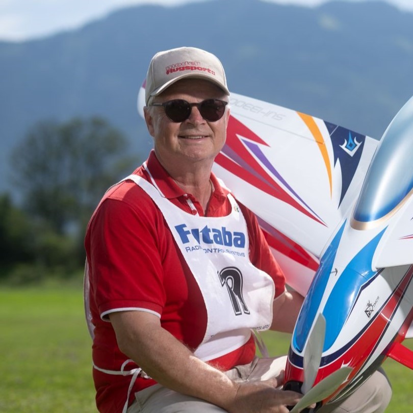 Matthias Bosshard
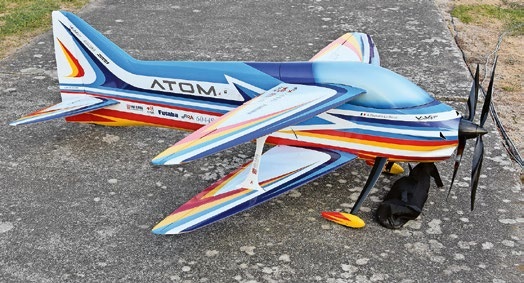
ATOM, THE NEW DOUBLE-DECKER FROM CPLR
Matthias Bosshard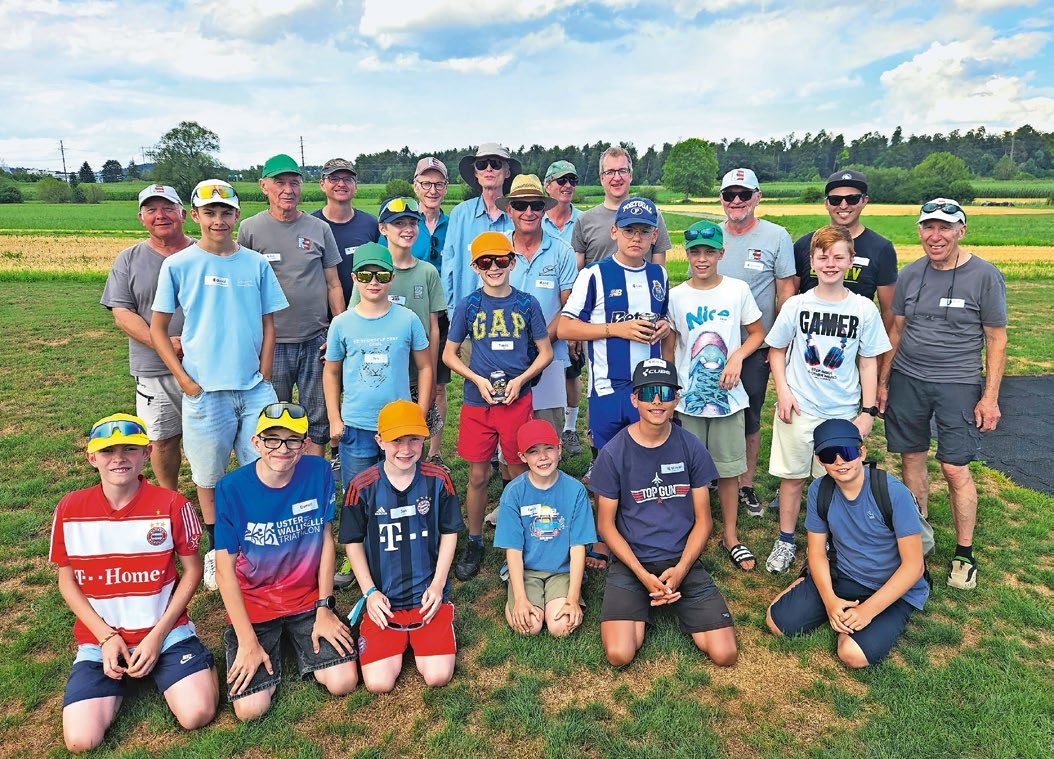
SUMMER FUN 2026 AT MG USTER
Martin Wunderli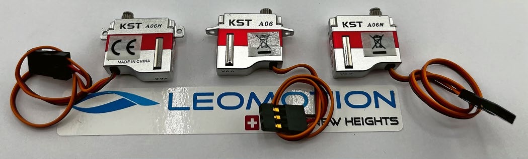
What's New at Leomotion.com
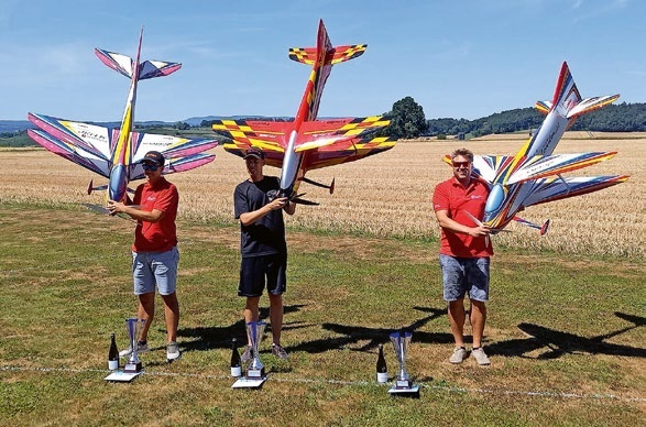
52. 2026 ALPS CUP
Emil Giezendanner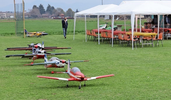
TWIN TOWN PARTNERSHIP
Wolfgang Voeller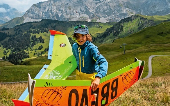
34th HAHNENMOOS ALPINE MODEL AIRPLANE CAMP
Res Dauwalder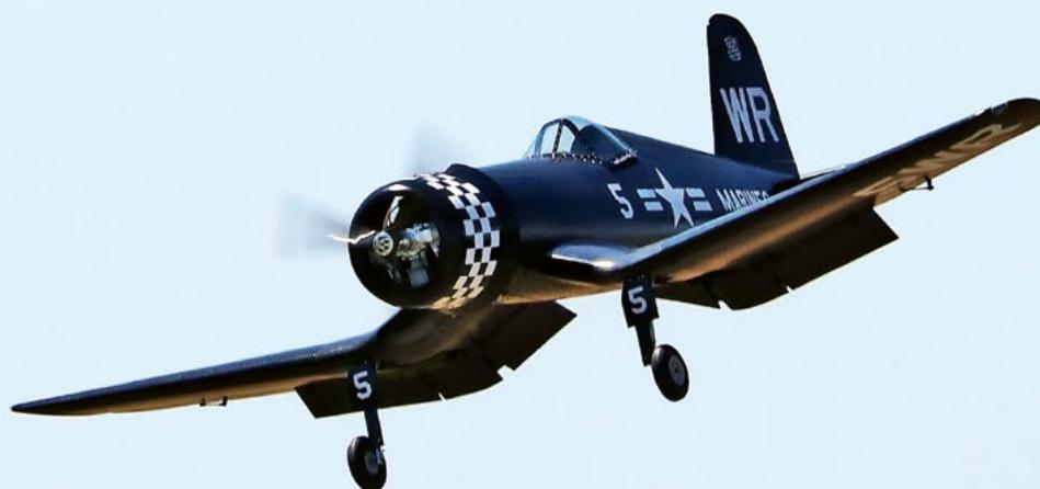
CORSAIR F4U – A WARBIRD WITH A MEMORABLE LOOK
Jürgen Rosenberger, Jürgen Prinz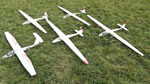
SMALL, MODEL-LIKE SAILBOATS
Res Dauwalder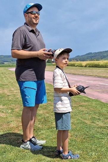
TRY-OUT DAY AT MFV WETTINGEN
Urs Keller
WELCOME, NEW MEMBER!
Andrea Bolliger
FREE FLIGHT IN THE MIDDLE OF SUMMER
Urs Muntwyler
COUPE DES ALPES – OBSERVE AND LEARN
Rodito Nussbaumer
EURO CONTEST GLIDER ACRO TOUR AUSTRIA 2026
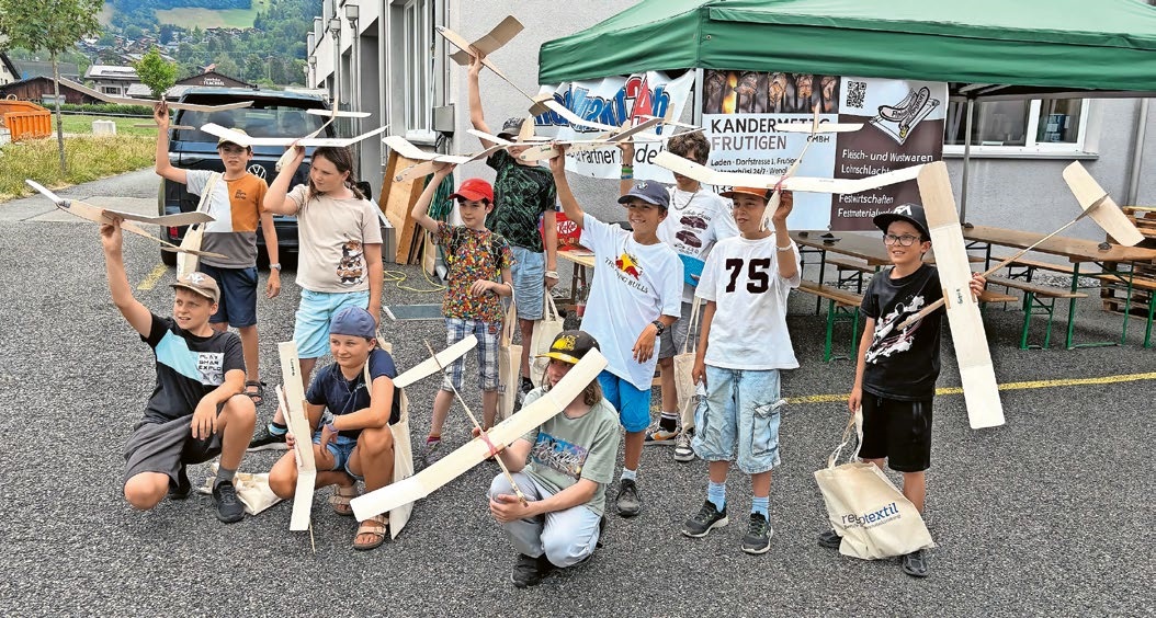
BY YOUTH, FOR YOUTH
Lorena Betschen
INSIGHTS INTO THE HISTORY OF SEAPLANES
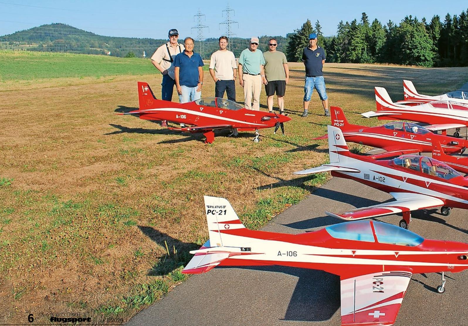
THE PC-21 STORY
Emil Giezendanner
NEWS FROM HEBU
 Julia Bucher
FROM 0 TO 100
Markus Nussbaumer
MEMORIES
Wolfgang Völler
NOS REGION – A HUB FOR ELECTRIC AVIATION
Emil Giezendanner
DO YOU KNOW WHAT I MEAN IN THE LAND OF SMILES?
Emil Giezendanner
Have you almost forgotten about aircraft that take off and land vertically?
Emil Giezendanner